Domination: The Relation That Makes Multi-Objective Optimization Work

In single-objective optimization, comparing two solutions is trivial: whichever has the lower cost wins. With multiple objectives, this breaks down immediately.

Say solution A costs $100 and takes 5 hours. Solution B costs $80 and takes 7 hours. Which is better? It depends on how much you value time versus money — and that’s a human judgment, not a mathematical one.

Multi-objective optimization doesn’t try to make that judgment. Instead, it identifies solutions that are unambiguously worse than some other solution. The concept that formalizes this is domination.

The Definition

Solution $a$ dominates solution $b$ (written $a \prec b$ ) if and only if:

$a$ is no worse than $b$ on every objective, and
$a$ is strictly better than $b$ on at least one objective.

Both conditions must hold. If $a$ wins on one objective but loses on another, neither dominates the other — they are non-dominated with respect to each other.

This is deliberately conservative. Domination only fires when one solution is unambiguously better. No weights, no preferences, no collapse of multiple objectives into a single score.

Show code

1
import numpy as np
2
import matplotlib.pyplot as plt
3
import matplotlib.patches as mpatches
4
from matplotlib.patches import FancyArrowPatch
5

6
np.random.seed(7)
7
plt.rcParams.update({
8
    'figure.dpi': 150,
9
    'font.family': 'sans-serif',
10
    'axes.spines.top': False,
11
    'axes.spines.right': False,
12
})

Four Cases

Given two solutions in a two-objective minimization problem, there are exactly four possible relationships. The plot below shows all of them from the perspective of the gray reference point.

Show code

1
ref = np.array([5.0, 5.0])
2

3
cases = [
4
    (np.array([3.0, 3.0]), '#16a34a', 'B dominates A\n(better on both)'),
5
    (np.array([7.0, 7.0]), '#dc2626', 'A dominates B\n(worse on both)'),
6
    (np.array([3.0, 7.0]), '#2563eb', 'Non-dominated\n(better f1, worse f2)'),
7
    (np.array([7.0, 3.0]), '#9333ea', 'Non-dominated\n(worse f1, better f2)'),
8
]
9

10
fig, axes = plt.subplots(1, 4, figsize=(14, 3.5), layout='constrained')
11

12
for ax, (pt, color, label) in zip(axes, cases):
13
    ax.scatter(*ref, color='#64748b', s=120, zorder=5, label='A (reference)')
14
    ax.scatter(*pt, color=color, s=120, zorder=5, marker='D', label='B')
15
    ax.annotate('A', ref, textcoords='offset points', xytext=(8, 4), fontsize=10, color='#64748b')
16
    ax.annotate('B', pt, textcoords='offset points', xytext=(8, 4), fontsize=10, color=color)
17
    ax.set_xlim(0, 10)
18
    ax.set_ylim(0, 10)
19
    ax.set_xlabel('f₁ (minimize)', fontsize=9)
20
    ax.set_ylabel('f₂ (minimize)', fontsize=9)
21
    ax.set_title(label, fontsize=9, color=color, fontweight='bold')
22
    ax.axvline(ref[0], color='#64748b', lw=0.8, linestyle='--', alpha=0.4)
23
    ax.axhline(ref[1], color='#64748b', lw=0.8, linestyle='--', alpha=0.4)
24

25
plt.suptitle('Domination cases relative to solution A', fontsize=11, fontweight='bold', y=1.02)
26
plt.sh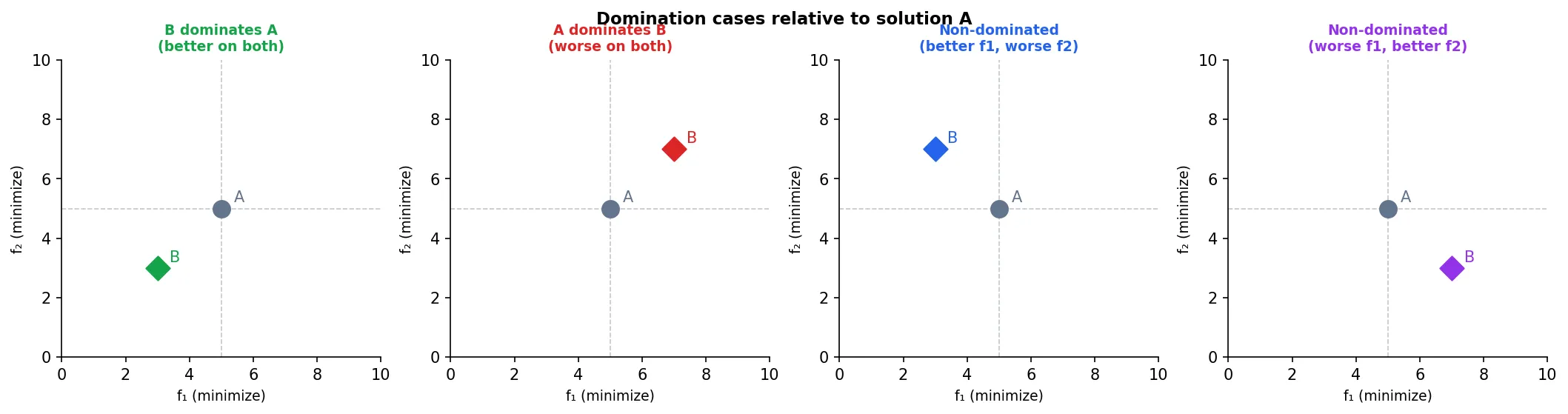ow()

The dashed lines partition the objective space into four quadrants relative to A:

Bottom-left: B dominates A — strictly better on both objectives.
Top-right: A dominates B — A is strictly better on both.
Bottom-right / Top-left: Neither dominates — one is better on f₁, the other on f₂.

The two non-dominated cases are exactly where value judgments are required. No algorithm can declare one solution better than the other without additional preference information.

Domination Depends on the Objective Direction

So far we’ve assumed both objectives are minimized. In practice, some objectives are maximized — profit, accuracy, coverage. The domination rule is the same, but the “better” direction flips.

For a minimization objective, lower is better. For a maximization objective, higher is better. The four combinations:

Show code

1
ref = np.array([5.0, 5.0])
2
b_pos = np.array([3.0, 3.0])  # always at same position; arrows show what 'better' means
3

4
cases = [
5
    ('min f₁,  min f₂', [(-1, 0), (0, -1)], '#2563eb'),
6
    ('min f₁,  max f₂', [(-1, 0), (0, +1)], '#16a34a'),
7
    ('max f₁,  min f₂', [(+1, 0), (0, -1)], '#9333ea'),
8
    ('max f₁,  max f₂', [(+1, 0), (0, +1)], '#dc2626'),
9
]
10

11
fig, axes = plt.subplots(2, 2, figsize=(10, 8), layout='constrained')
12
axes = axes.flatten()
13

14
for ax, (title, dirs, color) in zip(axes, cases):
15
    # Reference point A
16
    ax.scatter(*ref, color='#64748b', s=120, zorder=5)
17
    ax.annotate('A', ref, textcoords='offset points', xytext=(6, 4), fontsize=11, color='#64748b', fontweight='bold')
18

19
    # Shade the domination region (where B must lie to dominate A)
20
    dx, dy = dirs[0][0], dirs[1][1]
21
    x0 = ref[0] if dx < 0 else 0
22
    x1 = ref[0] if dx > 0 else 10
23
    y0 = ref[1] if dy < 0 else 0
24
    y1 = ref[1] if dy > 0 else 10
25
    # Strict dominance region (excluding the ref lines themselves)
26
    ax.fill_between([x0, x1], [y0, y0], [y1, y1], color=color, alpha=0.12, zorder=1)
27

28
    # Example dominating point B
29
    bx = ref[0] - 1.8 * dx
30
    by = ref[1] - 1.8 * dy
31
    ax.scatter(bx, by, color=color, s=120, zorder=5, marker='D')
32
    ax.annotate('B (dominates A)', (bx, by), textcoords='offset points', xytext=(6, 4), fontsize=9, color=color)
33

34
    # Crosshair through A
35
    ax.axvline(ref[0], color='#64748b', lw=0.8, linestyle='--', alpha=0.5)
36
    ax.axhline(ref[1], color='#64748b', lw=0.8, linestyle='--', alpha=0.5)
37

38
    # Direction arrows on axes
39
    arrow_kw = dict(arrowstyle='->', color='#94a3b8', lw=1.2)
40
    if dx < 0:
41
        ax.annotate('', xy=(1, 0.5), xytext=(9, 0.5), arrowprops=arrow_kw)
42
        ax.text(0.5, 0.2, 'better →', fontsize=7, color='#94a3b8', rotation=0)
43
    else:
44
        ax.annotate('', xy=(9, 0.5), xytext=(1, 0.5), arrowprops=arrow_kw)
45
        ax.text(8, 0.2, '← better', fontsize=7, color='#94a3b8')
46
    if dy < 0:
47
        ax.annotate('', xy=(0.5, 1), xytext=(0.5, 9), arrowprops=arrow_kw)
48
        ax.text(0.1, 0.5, 'better', fontsize=7, color='#94a3b8', rotation=90)
49
    else:
50
        ax.annotate('', xy=(0.5, 9), xytext=(0.5, 1), arrowprops=arrow_kw)
51
        ax.text(0.1, 8, 'better', fontsize=7, color='#94a3b8', rotation=90)
52

53
    ax.set_xlim(0, 10)
54
    ax.set_ylim(0, 10)
55
    ax.set_xlabel('f₁', fontsize=11)
56
    ax.set_ylabel('f₂', fontsize=11)
57
    ax.set_title(title, fontsize=11, fontweight='bold', color=color)
58

59
plt.suptitle('Domination region (shaded) depends on objective directions', fontsize=12, fontweight='bold')
60
plt.sh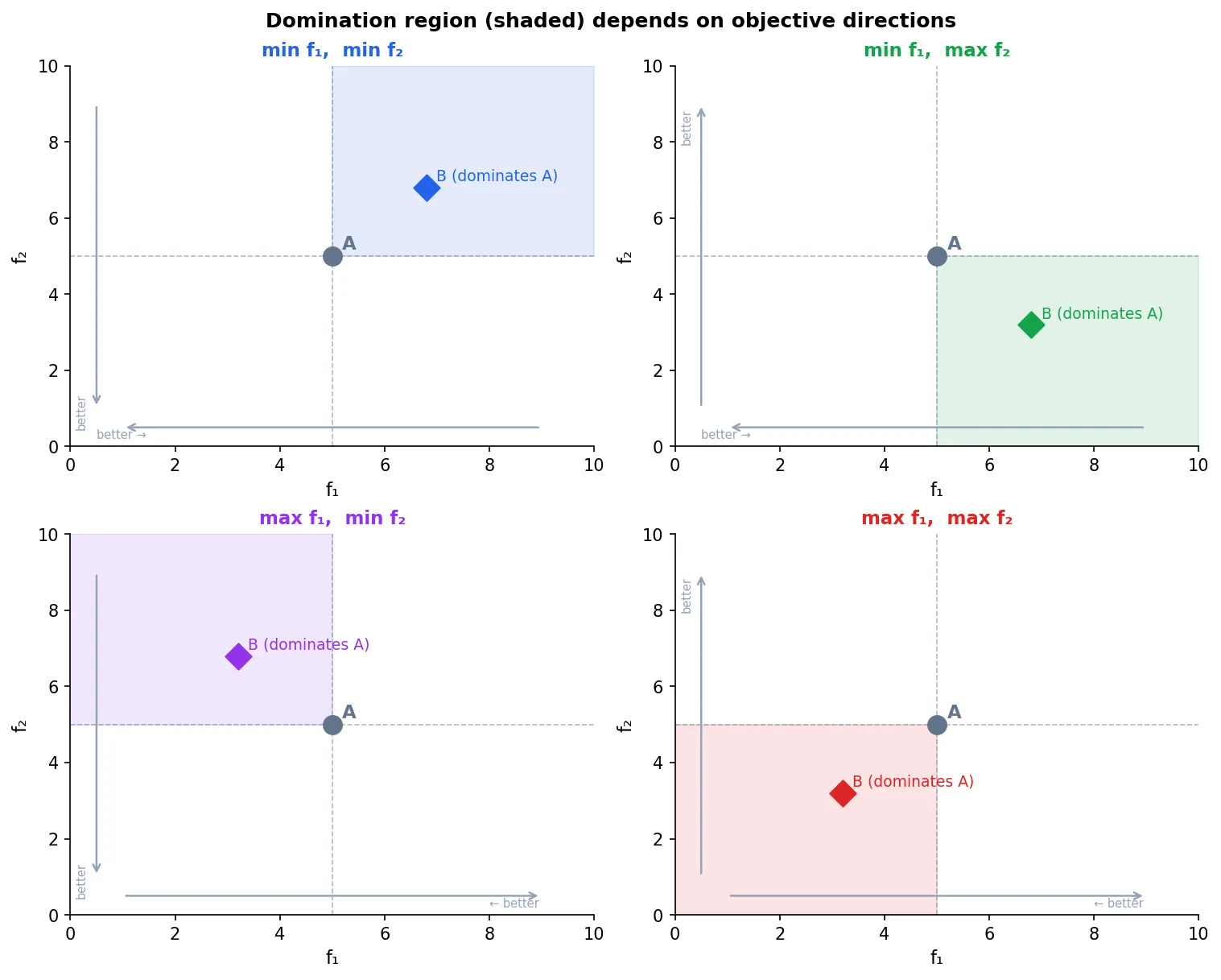ow()

The shaded region shows where B must lie to dominate A. The reference point A sits at the corner — B needs to be strictly inside the shaded region on at least one axis and no worse on any other.

In code, the only change needed is flipping the comparison sign for maximized objectives:

1
# directions: -1 = minimize, +1 = maximize
2
def dominates(a, b, directions):
3
    # Convert to minimization: multiply by direction
4
    a_norm = a * directions
5
    b_norm = b * directions
6
    return np.all(a_norm <= b_norm) and np.any(a_norm < b_norm)

Multiplying by the direction vector maps every maximization objective to minimization, so the standard domination check applies uniformly. Most multi-objective frameworks — including pymoo — handle this internally by convention (pymoo always minimizes; to maximize, negate the objective).

In a Population

With many solutions, we apply domination pairwise. A solution is non-dominated if no other solution in the population dominates it. The set of all non-dominated solutions is the Pareto front — the topic of the next post.

Here’s a population where each point is colored by whether it’s dominated or not.

Show code

1
def dominates(a, b):
2
    """Return True if a dominates b (minimization)."""
3
    return np.all(a <= b) and np.any(a < b)
4

5
def non_dominated_mask(costs):
6
    n = len(costs)
7
    dominated = np.zeros(n, dtype=bool)
8
    for i in range(n):
9
        for j in range(n):
10
            if i != j and dominates(costs[j], costs[i]):
11
                dominated[i] = True
12
                break
13
    return ~dominated
14

15
n = 60
16
pop = np.random.rand(n, 2) * 10
17
mask = non_dominated_mask(pop)
18

19
fig, ax = plt.subplots(figsize=(7, 5), layout='constrained')
20
ax.scatter(pop[~mask, 0], pop[~mask, 1], color='#94a3b8', alpha=0.6, s=45, label='Dominated')
21
ax.scatter(pop[mask, 0], pop[mask, 1], color='#2563eb', s=70, zorder=5, label='Non-dominated (Pareto front)')
22

23
front = pop[mask]
24
front = front[front[:, 0].argsort()]
25
ax.step(front[:, 0], front[:, 1], where='post', color='#2563eb', alpha=0.35, lw=1.5)
26

27
ax.set_xlabel('f₁ (minimize)', fontsize=12)
28
ax.set_ylabel('f₂ (minimize)', fontsize=12)
29
ax.set_title('Non-dominated solutions in a population', fontsize=13, fontweight='bold')
30
ax.legend(frameon=False)
31
plt.sh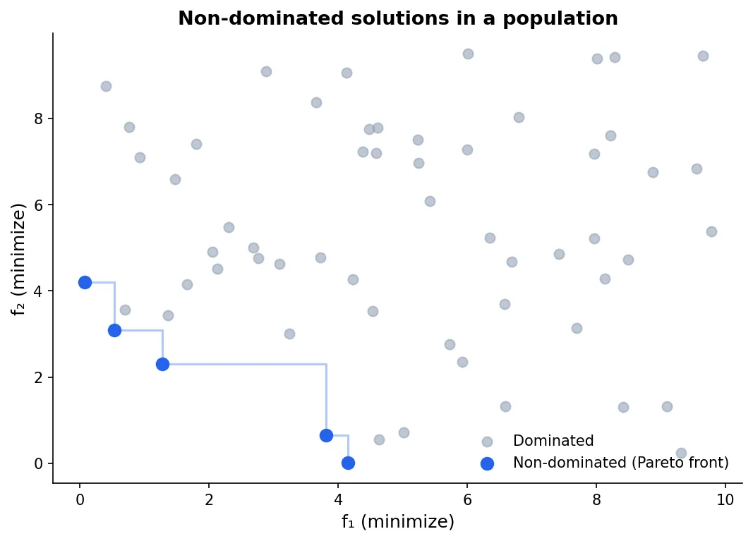ow()

The Complexity Problem

The naive algorithm above is $O(n^2 \cdot m)$ where $n$ is the population size and $m$ is the number of objectives. For small populations this is fine. For large $n$ or many objectives it becomes a bottleneck.

There are faster algorithms — the most well-known being the fast non-dominated sort from NSGA-II, which runs in $O(n^2 \cdot m)$ worst case but organizes solutions into fronts (rank 1 = non-dominated, rank 2 = non-dominated after removing rank 1, and so on). This ranking is what drives selection in most evolutionary multi-objective algorithms.

There’s also a deeper issue: as the number of objectives grows, domination becomes less useful. In high dimensions, almost every solution is non-dominated with respect to every other — the front encompasses the entire population. This is the curse of dimensionality for multi-objective optimization, and it’s why algorithms for many-objective problems ( $m \geq 4$ ) need fundamentally different mechanisms beyond domination alone.

For two and three objectives, domination works well and the Pareto front is geometrically meaningful. That’s the regime where most practical problems live.

Summary

Domination is the foundational comparison relation in multi-objective optimization. It identifies when one solution is unambiguously better than another — without requiring weights or preference information. Solutions that no other solution dominates form the Pareto front.

The next post looks at the Pareto front itself: what it represents geometrically, how its shape encodes the structure of the trade-off, and what it means to “solve” a multi-objective problem.

Domination: The Relation That Makes Multi-Objective Optimization Work

The Definition

Four Cases

Domination Depends on the Objective Direction

In a Population

The Complexity Problem

Summary

Related Posts

Two Ways to Solve a Multi-Objective Problem

The Pareto Front