The Pareto Front

Most optimization problems taught in school have a single objective: minimize cost, maximize profit, find the shortest path. Clean, tractable, satisfying.

Real problems rarely look like that.

In practice you’re almost always balancing competing goals. A logistics network that minimizes cost will sacrifice service speed. A model that maximizes accuracy will sacrifice interpretability. A schedule that maximizes throughput will sacrifice flexibility. When two objectives genuinely conflict, there is no single best solution — only trade-offs.

The Pareto front is the mathematical object that makes those trade-offs explicit.

1
import numpy as np
2
import matplotlib.pyplot as plt
3

4
np.random.seed(42)
5
plt.rcParams.update({
6
    'figure.dpi': 150,
7
    'font.family': 'sans-serif',
8
    'axes.spines.top': False,
9
    'axes.spines.right': False,
10
})

What It Is

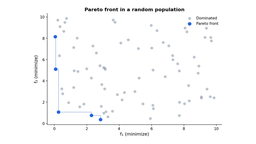
Given a set of candidate solutions, each evaluated on two or more objectives, a solution is non-dominated if no other solution is better on all objectives simultaneously. The Pareto front is the set of all non-dominated solutions.

Any solution not on the Pareto front is dominated — there is some other solution that is at least as good on every objective and strictly better on at least one. A rational decision-maker would never choose a dominated solution.

The code below computes this for a random population with two objectives.

1
def non_dominated_mask(costs):
2
    n = len(costs)
3
    dominated = np.zeros(n, dtype=bool)
4
    for i in range(n):
5
        for j in range(n):
6
            if i != j:
7
                if np.all(costs[j] <= costs[i]) and np.any(costs[j] < costs[i]):
8
                    dominated[i] = True
9
                    break
10
    return ~dominated
11

12
n = 80
13
solutions = np.random.rand(n, 2) * 10
14
mask = non_dominated_mask(solutions)
15

16
front = solutions[mask]
17
front = front[front[:, 0].argsort()]
18

19
fig, ax = plt.subplots(figsize=(7, 5), layout='constrained')
20
ax.scatter(solutions[~mask, 0], solutions[~mask, 1],
21
           color='#94a3b8', alpha=0.6, s=40, label='Dominated')
22
ax.scatter(front[:, 0], front[:, 1],
23
           color='#2563eb', s=70, zorder=5, label='Pareto front')
24
ax.step(front[:, 0], front[:, 1], where='post',
25
        color='#2563eb', alpha=0.4, linewidth=1.5)
26

27
ax.set_xlabel('f₁ (minimize)', fontsize=12)
28
ax.set_ylabel('f₂ (minimize)', fontsize=12)
29
ax.set_title('Pareto front in a random population', fontsize=13, fontweight='bold')
30
ax.legend(frameon=False)
31
plt.sh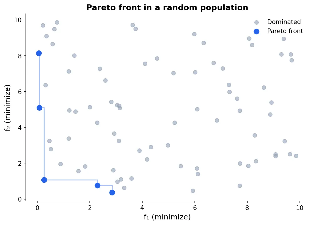ow()

What the Shape Tells You

The Pareto front is not just a set of solutions — its shape encodes the structure of the trade-off.

A convex front means the trade-off is smooth and roughly linear: giving up a unit of f₁ buys roughly a constant improvement in f₂ across the front. A concave front means the trade-off has diminishing returns in the middle — the extreme solutions are strong, but compromises are relatively costly. A disconnected front means there are regions of objective space that simply can’t be achieved by any feasible solution.

The shape also determines which algorithms can find the front. As shown in the next post, the weighted sum method can only recover points on a convex front — it systematically misses concave regions regardless of how you set the weights.

1
t = np.linspace(0, 1, 200)
2

3
fronts = {
4
    'Convex': np.column_stack([t, (1 - t**2)**0.5]),
5
    'Concave': np.column_stack([t, 1 - t**0.5]),
6
    'Linear': np.column_stack([t, 1 - t]),
7
}
8

9
colors = ['#2563eb', '#dc2626', '#16a34a']
10

11
fig, axes = plt.subplots(1, 3, figsize=(12, 4), layout='constrained')
12
for ax, (name, front_pts), color in zip(axes, fronts.items(), colors):
13
    ax.plot(front_pts[:, 0], front_pts[:, 1], color=color, lw=2.5)
14
    ax.set_xlim(-0.05, 1.1)
15
    ax.set_ylim(-0.05, 1.1)
16
    ax.set_xlabel('f₁', fontsize=11)
17
    ax.set_ylabel('f₂', fontsize=11)
18
    ax.set_title(name, fontsize=12, fontweight='bold', color=color)
19
    ax.set_aspect('equal')
20

21
plt.suptitle('Pareto front shapes', fontsize=12, fontweight='bold')
22
plt.sh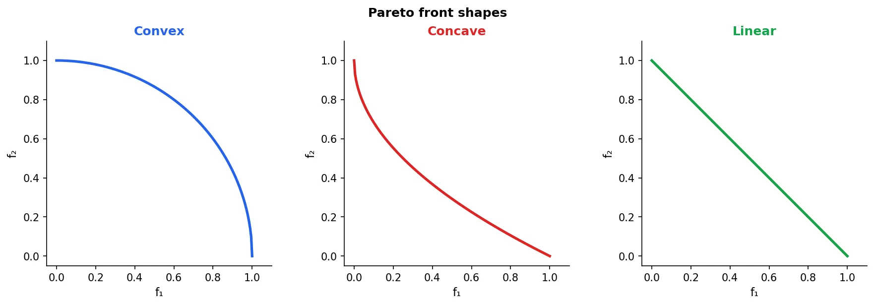ow()

Optimization vs. Decision-Making

Finding the Pareto front is an optimization problem. Choosing a point on it is a decision problem — and they are fundamentally different.

The optimization algorithm doesn’t know which trade-off is acceptable. That depends on business context, stakeholder priorities, and constraints that aren’t in the objective functions. The right workflow is:

1. Compute (an approximation of) the Pareto front.
2. Present it to decision-makers — ideally as an interactive plot, not just a table of numbers.
3. Let them choose the solution that matches their priorities.

Collapsing step 1 and 3 — choosing weights upfront and returning a single solution — only makes sense when the preference structure is genuinely known in advance. In practice, stakeholders often don’t know their preferences until they see the options. The Pareto front gives them that information.

What’s Next

The next post in this series compares the two main approaches to computing the Pareto front: the weighted sum method and evolutionary algorithms like NSGA-II. They make different assumptions and return different things — and knowing when to use which is practical knowledge that most introductions skip.