· Julian Blank · 7 min read
Two Ways to Solve a Multi-Objective Problem
The weighted sum method and evolutionary algorithms both claim to solve multi-objective problems. They're doing fundamentally different things — and the difference matters for what you get out.
There are two dominant philosophies for handling multiple objectives in optimization.
The first says: collapse the objectives into one by assigning weights, then solve a single-objective problem. Simple, fast, and works with any existing solver.
The second says: keep the objectives separate, evolve a population of solutions simultaneously, and return the full trade-off frontier in one run.
Both approaches are correct in their own terms. They answer different questions — and which one you should use depends on what you actually need.
Show code
import numpy as npimport matplotlib.pyplot as pltfrom matplotlib.colors import Normalizefrom matplotlib.cm import ScalarMappablefrom pymoo.core.problem import Problemfrom pymoo.algorithms.moo.nsga2 import NSGA2from pymoo.optimize import minimize as pymoo_minimize
np.random.seed(0)plt.rcParams.update({ 'figure.dpi': 150, 'font.family': 'sans-serif', 'axes.spines.top': False, 'axes.spines.right': False,})The Weighted Sum
The weighted sum scalarizes a multi-objective problem into a single scalar:
with and . Each weight encodes relative importance. Once the problem is scalar, any off-the-shelf solver applies.
If you run this repeatedly with different weight vectors, each run returns one point on (or near) the Pareto front. The plot below shows this: each weight produces a different optimal solution, and sweeping across weights traces out the front.
Show code
# Convex Pareto front: f1^2 + f2^2 = 1 in the first quadranttheta = np.linspace(0, np.pi / 2, 300)true_front = np.column_stack([np.cos(theta), np.sin(theta)])
# For weighted sum on a convex front, optimal point given weight w is:# minimize w*f1 + (1-w)*f2 subject to f1^2+f2^2=1# Solution: f1 = w/sqrt(w^2+(1-w)^2), f2 = (1-w)/sqrt(w^2+(1-w)^2)weights = np.linspace(0.05, 0.95, 12)ws_points = np.array([ [w / np.sqrt(w**2 + (1-w)**2), (1-w) / np.sqrt(w**2 + (1-w)**2)] for w in weights])
fig, ax = plt.subplots(figsize=(6, 5), layout='constrained')ax.plot(true_front[:, 0], true_front[:, 1], color='#94a3b8', lw=1.5, label='True Pareto front')
cmap = plt.cm.Bluesnorm = Normalize(vmin=0, vmax=1)for i, (pt, w) in enumerate(zip(ws_points, weights)): ax.scatter(*pt, color=cmap(norm(w)), s=80, zorder=5)
sm = ScalarMappable(cmap=cmap, norm=norm)sm.set_array([])cbar = plt.colorbar(sm, ax=ax, fraction=0.035, pad=0.02)cbar.set_label('weight w₁', fontsize=9)
ax.set_xlabel('f₁ (minimize)', fontsize=12)ax.set_ylabel('f₂ (minimize)', fontsize=12)ax.set_title('Weighted sum: each weight → one solution', fontsize=12, fontweight='bold')ax.legend(frameon=False, fontsize=9)plt.show()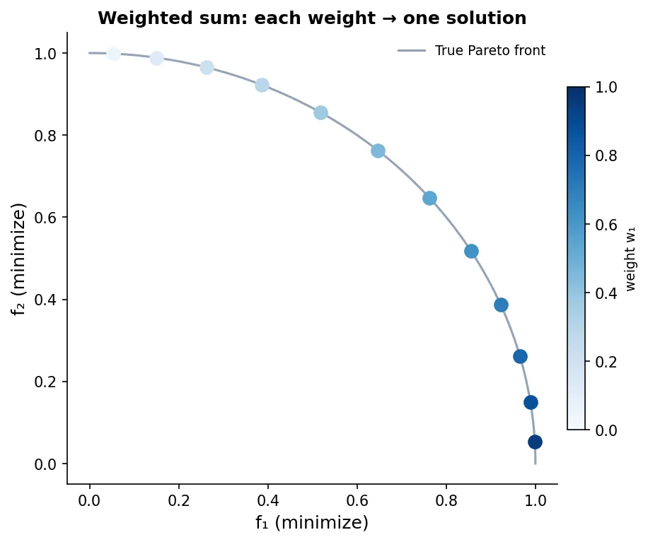
On a convex front this works perfectly — every point is reachable by some weight vector. But real problems rarely have convex fronts.
On a non-convex or disconnected front, the weighted sum has a fundamental limitation: entire regions of the Pareto front are unreachable, no matter what weights you choose. The weight vector steers the solver toward a region, but if that region is concave, the solver skips over it and lands elsewhere.
Show code
# Non-convex front: bump in the middlet = np.linspace(0, 1, 300)f1 = tf2 = (1 - t**0.5)**2 # non-convextrue_front_nc = np.column_stack([f1, f2])
# Weighted sum can only reach points on the convex hull of the front# The reachable region is the line connecting (0,1) and (1,0)ws_f1 = np.linspace(0.05, 0.95, 12)ws_f2 = 1 - ws_f1 # convex hull of this front is just the line
# Find closest front point for each ws solution (projection)ws_pts = []for w in weights: scores = w * f1 + (1 - w) * f2 idx = np.argmin(scores) ws_pts.append([f1[idx], f2[idx]])ws_pts = np.array(ws_pts)
fig, ax = plt.subplots(figsize=(6, 5), layout='constrained')ax.plot(true_front_nc[:, 0], true_front_nc[:, 1], color='#94a3b8', lw=1.5, label='True Pareto front')ax.scatter(ws_pts[:, 0], ws_pts[:, 1], color='#2563eb', s=80, zorder=5, label='Weighted sum solutions')
# Shade the unreachable regionmid_t = np.linspace(0.1, 0.9, 200)mid_f1 = mid_tmid_f2_front = (1 - mid_t**0.5)**2mid_f2_line = 1 - mid_tax.fill_between(mid_f1, mid_f2_front, mid_f2_line, color='#fca5a5', alpha=0.35, label='Unreachable by weighted sum')
ax.set_xlabel('f₁ (minimize)', fontsize=12)ax.set_ylabel('f₂ (minimize)', fontsize=12)ax.set_title('Non-convex front: weighted sum misses solutions', fontsize=12, fontweight='bold')ax.legend(frameon=False, fontsize=9)plt.show()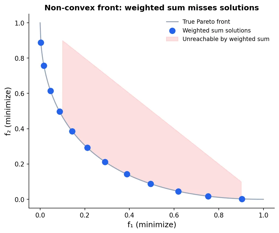
Evolutionary Algorithms
Evolutionary multi-objective algorithms (EMOAs) take a different approach: instead of scalarizing and solving once, they maintain a population of solutions and evolve it toward the full Pareto front simultaneously.
The dominant algorithm in this class is NSGA-II (Non-dominated Sorting Genetic Algorithm II). Its selection mechanism has two components:
- Non-dominated rank: solutions on the Pareto front are rank 1, solutions non-dominated after removing rank 1 are rank 2, and so on. Lower rank is preferred.
- Crowding distance: among solutions of equal rank, prefer those in less crowded regions of the front. This maintains diversity and prevents the algorithm from converging to a single point.
The result after enough generations is a population spread across the Pareto front — including concave regions that the weighted sum cannot reach.
Show code
# Define the non-convex problem: f1=x, f2=(1-sqrt(x))^2, x in [0,1]class NonConvexProblem(Problem): def __init__(self): super().__init__(n_var=1, n_obj=2, xl=0.0, xu=1.0)
def _evaluate(self, x, out, *args, **kwargs): f1 = x[:, 0] f2 = (1 - np.sqrt(x[:, 0])) ** 2 out["F"] = np.column_stack([f1, f2])
res = pymoo_minimize( NonConvexProblem(), NSGA2(pop_size=60), ('n_gen', 120), seed=1, verbose=False,)
t = np.linspace(0, 1, 300)true_front_nc = np.column_stack([t, (1 - np.sqrt(t)) ** 2])
weights = np.linspace(0.05, 0.95, 12)ws_pts = []for w in weights: scores = w * t + (1 - w) * (1 - np.sqrt(t)) ** 2 idx = np.argmin(scores) ws_pts.append([t[idx], (1 - np.sqrt(t[idx])) ** 2])ws_pts = np.array(ws_pts)
mid_t = np.linspace(0.05, 0.95, 200)mid_f2_front = (1 - np.sqrt(mid_t)) ** 2mid_f2_line = 1 - mid_t
fig, axes = plt.subplots(1, 2, figsize=(12, 5), layout='constrained')
for ax in axes: ax.plot(true_front_nc[:, 0], true_front_nc[:, 1], color='#94a3b8', lw=1.5, label='True Pareto front', zorder=1) ax.set_xlabel('f₁ (minimize)', fontsize=11) ax.set_ylabel('f₂ (minimize)', fontsize=11) ax.set_xlim(-0.05, 1.1) ax.set_ylim(-0.05, 1.1)
axes[0].scatter(ws_pts[:, 0], ws_pts[:, 1], color='#2563eb', s=70, zorder=5, label='Weighted sum (12 runs)')axes[0].fill_between(mid_t, mid_f2_front, mid_f2_line, color='#fca5a5', alpha=0.3, label='Unreachable')axes[0].set_title('Weighted Sum', fontsize=12, fontweight='bold')axes[0].legend(frameon=False, fontsize=9)
axes[1].scatter(res.F[:, 0], res.F[:, 1], color='#16a34a', s=70, zorder=5, alpha=0.8, label=f'NSGA-II (pymoo, {len(res.F)} solutions)')axes[1].set_title('NSGA-II via pymoo', fontsize=12, fontweight='bold')axes[1].legend(frameon=False, fontsize=9)
plt.suptitle('Approximating the Pareto front: two approaches', fontsize=12, fontweight='bold')plt.show()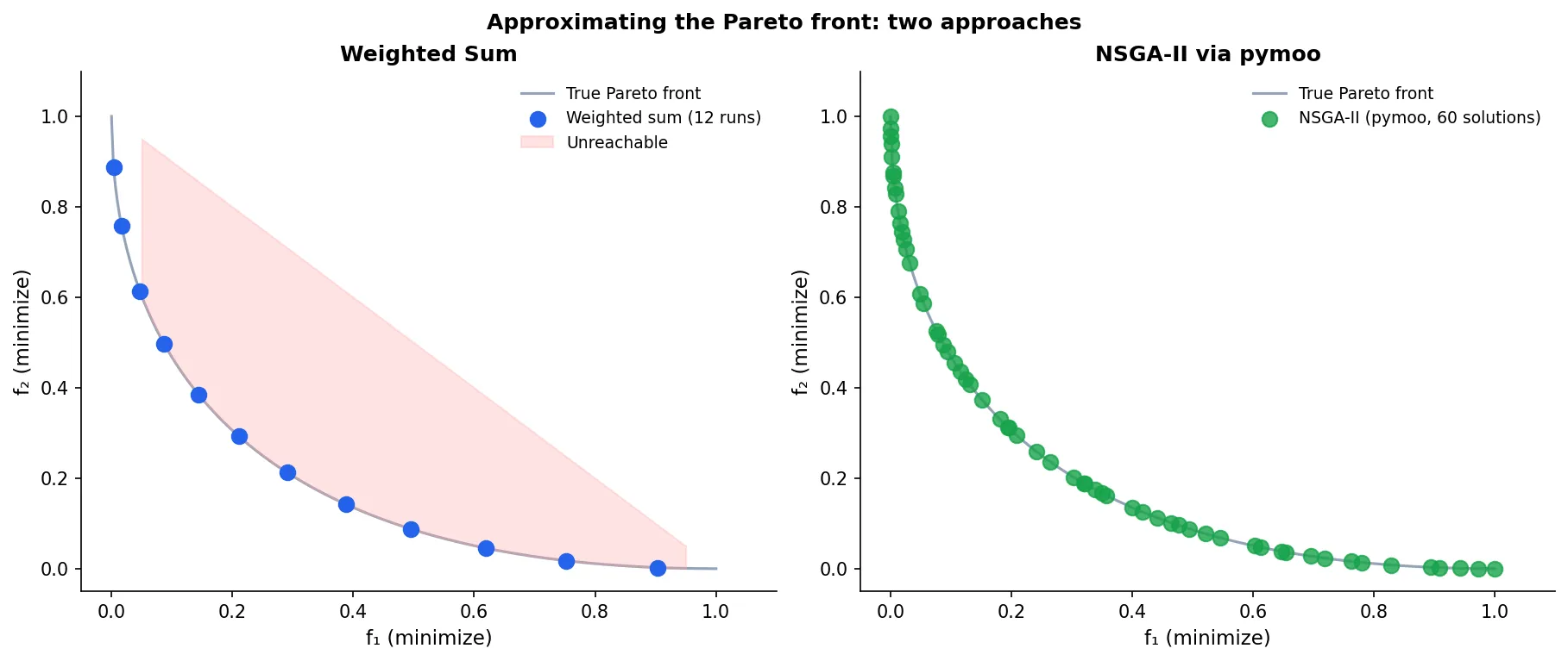
When to Use Which
These two approaches make different trade-offs, and the right choice depends on the problem.
Use the weighted sum when:
- You already know the weights — a stakeholder can tell you that cost matters twice as much as time.
- You need a single solution fast and you know the front is approximately convex.
- You’re embedding the multi-objective problem inside a larger system and need differentiability (the weighted sum is smooth if the objectives are).
- You want to use a classical solver (LP, QP, gradient descent) that doesn’t understand populations.
Use an evolutionary algorithm when:
- You don’t know the weights in advance and want to present decision-makers with options.
- The front is non-convex or disconnected and you need solutions from those regions.
- The objectives are black-box functions with no gradient information.
- You want one run to return the full trade-off picture rather than a single point.
The cost of evolutionary algorithms is computational: they require many function evaluations (typically hundreds to thousands). For cheap-to-evaluate functions this is fine. For expensive simulations — say, a computational fluid dynamics solver — each evaluation costs minutes, and you need to think harder about whether to run an evolutionary algorithm at all or use a surrogate model.
The Deeper Point
The weighted sum and evolutionary algorithms are not competing methods — they’re answering different questions.
The weighted sum asks: given these preferences, what’s the best solution? It requires you to specify preferences upfront.
The evolutionary approach asks: what are all the defensible solutions, independent of preferences? It defers the preference question to the decision-maker after seeing the options.
In practice, most serious multi-objective work uses evolutionary algorithms to generate the front, then applies structured decision-making to select from it. The two phases — optimization and decision-making — are kept separate, and for good reason: conflating them hides information that the decision-maker needs.